Advanced Topics in Machine Learning - CST396 KTU CS Sixth Semester Honours Course - Dr Binu V P

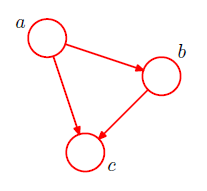
Probabilities play a central role in modern pattern recognition.it highly advantageous to augment the analysis using diagrammatic representations of probability distributions, called probabilistic graphical models. These offer several useful properties 1. They provide a simple way to visualize the structure of a probabilistic model and can be used to design and motivate new models. 2. Insights into the properties of the model, including conditional independence properties, can be obtained by inspection of the graph. 3. Complex computations, required to perform inference and learning in sophisticated models, can be expressed in terms of graphical manipulations, in which underlying mathematical expressions are carried along implicitly. A graph comprises nodes (also called vertices) connected by links (also known as edges or arcs). In a probabilistic graphical model, each node represents a random variable (or group of random variables), and the links express probabilistic relationship

 Syllabus Module -1 (Supervised Learning) Overview of machine learning - supervised, semi-supervised, unsupervised learning, reinforcement learning Regression algorithms: least squares linear regression, gradient descent, closed form, normal equations, regularization techniques (LASSO, RIDGE), polynomial regression. Discriminative Methods - Logistic Regression, Decision Tree Learning. Generative Methods - Naive Bayes Classifier, Gaussian Discriminant Analysis (GDA). Module -2 (Unsupervised Learning) Clustering - Similarity measures, Hierarchical Agglomerative Clustering, K-means partitional clustering, K-medoids clustering, Gaussian mixture models: Expectation Maximization (EM) algorithm for Gaussian mixture model Module -3 (Practical aspects in machine learning) Classification Performance measures - Precision, Recall, Accuracy, F-Measure, ROC, AUC, generalisation and overfitting, cross-validation, bias-variance tradeoff, error estimation, parameter and model selection. Ensemble Method

There are two types of Supervised Learning algorithms used for classification in Machine Learning. Discriminative Learning Algorithms Generative Learning Algorithms Discriminative Learning Algorithms include Logistic Regression, Perceptron Algorithm, etc. which try to find a decision boundary between different classes during the learning process. For example, given a classification problem to predict whether a patient has malaria or not, a Discriminative Learning Algorithm will try to create a classification boundary to separate two types of patients, and when a new example is introduced it is checked on which side of the boundary the example lies to classify it. Such algorithms try to model $P(y|X)$ i.e. given a feature set $X$ for a data sample what is the probability it belongs to the class ‘$y$’.Learning algorithms that model $P(y|X; θ)$, the conditional distribution of $y$ given $x$. For instance, logistic regression modeled $P(y|X; \theta)$ as $h_\theta(x) = g(\theta^ T x)$ wh

K-Medoids (also called Partitioning Around Medoid) algorithm was proposed in 1987 by Kaufman and Rousseeuw. A medoid can be defined as a point in the cluster, whose dissimilarities with all the other points in the cluster are minimum. The dissimilarity of the $medoid(C_i)$ and $object(P_i)$ is calculated by using $E = |P_i – C_i|$ The cost in K-Medoids algorithm is given as $C=\sum_{C_i} \sum_{P_i \in C_i} |P_i-C_i|$ Algorithm 1.Initialize: select $k$ random points out of the $n$ data points as the medoids. 2.Associate each data point to the closest medoid by using any common distance metric methods. 3.While the cost decreases: For each medoid $m$, for each data point  $o$ which is not a medoid:       Swap $m$ and $o$, associate each data point to the closest medoid, and recompute the cost.      If the total cost is more than that in the previous step, undo the swap. Let’s consider the following example: If a graph is drawn using the above data points, we obtain the following: Step

Probably Approximately Correct (PAC) learning framework. PAC (Probably Approximately Correct) learning is a framework used for mathematical analysis. A PAC Learner tries to learn a concept (approximately correct) by selecting a hypothesis from a set of hypotheses that has a low generalization error. In the context of Machine Learning, a problem is PAC-learnable if there is an algorithm $A$ when given some independently drawn samples, will produce a hypothesis with a small error for any distribution $D$ and any concept $c$, and that too with a high probability. It may not be possible to find a perfect hypothesis with zero error so the goal is to find a consistent hypothesis that can predict approximately correctly with an upper bound on the error.The PAC learning framework was introduced by Valiant [1984]. Motivation   Some computational learning questions  • What can be learned efficiently?  • What is inherently hard to learn?  • A general model of learning?  Complexity   • Computat

The hypothesis sets typically used in machine learning are infinite. But the sample complexity bounds of the previous discussions are uninformative when dealing with infinite hypothesis sets. One could ask whether efficient learning from a infinite sample is even possible when the hypothesis set $H$ is infinite. Our analysis of the family of axis-aligned rectangles  indicates that this is indeed possible at least in some cases, since we proved that that infinite concept class was PAClearnable. Our goal here will be to generalize that result and derive general learning guarantees for infinite hypothesis sets.A general idea for doing so consists of reducing the infinite case to the analysis of infinite sets of hypotheses and then proceed as in the finite case. There are different techniques for that reduction, each relying on a different notion of complexity for the family of hypotheses. The first complexity notion we will use is that of Rademacher complexity. This will help us derive