Discriminative and Generative Algorithms

There are two types of Supervised Learning algorithms used for classification in Machine Learning.

Discriminative Learning Algorithms

Generative Learning Algorithms

Discriminative Learning Algorithms include Logistic Regression, Perceptron Algorithm, etc. which try to find a decision boundary between different classes during the learning process. For example, given a classification problem to predict whether a patient has malaria or not, a Discriminative Learning Algorithm will try to create a classification boundary to separate two types of patients, and when a new example is introduced it is checked on which side of the boundary the example lies to classify it. Such algorithms try to model $P(y|X)$ i.e. given a feature set $X$ for a data sample what is the probability it belongs to the class ‘$y$’.Learning algorithms that model $P(y|X; θ)$, the conditional distribution of $y$ given $x$. For instance, logistic regression modeled $P(y|X; \theta)$ as $h_\theta(x) = g(\theta^ T x)$ where $g$ is the sigmoid function.

On the other hand, Generative Learning Algorithms follow a different approach, they try to capture the distribution of each class separately instead of finding a decision boundary among classes. Considering the previous example, a Generative Learning Algorithm will look at the distribution of infected patients and healthy patients separately and try to learn each of the distribution’s features separately, when a new example is introduced it is compared to both the distributions, the class to which the data example resembles the most will be assigned to it. Such algorithms try to model $P(X|y)$ for a given $P(y)$ here, $P(y)$ is known as a class prior.

The predictions for generative learning algorithms are made using Bayes Theorem as follows:

$P(y|X)=\frac{P(X|y)P(y)}{P(X)}$

where $P(X)=P(X|y=1).P(y=1)+P(X|y=0).P(y=0)$

Using only the values of $P(X|y)$ and $P(y)$ for the particular class we can calculate $P(y|X)$ i.e given the features of a data sample what is the probability it belongs to the class ‘$y$’.

Actually, if we are calculating $P(y|X)$ in order to make a prediction, then we don’t actually need to calculate the denominator, since 

$arg max_y P(y|X) = arg max_y P(X|y)P(y)$

$P(X) = arg max_y P(X|y)P(y)$

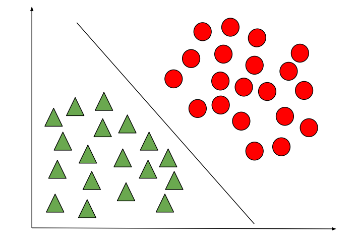
The below images depict the difference between the Discriminative and Generative Learning Algorithms. The probability of a prediction in the case of the Generative learning algorithm will be high if it lies near the centre of the contour corresponding to its class and decreases as we move away from the centre of the contour.

Gaussian Discriminant Analysis

GDA is a Generative Learning Algorithm and in order to capture the distribution of each class, it tries to fit a Gaussian Distribution to every class of the data separately. In this model, we’ll assume that $p(X|y)$ is distributed according to a multivariate normal distribution. Let’s talk briefly about the properties of multivariate normal distributions before moving on to the GDA model itself. 

The multivariate normal distribution The multivariate normal distribution in $d$-dimensions, also called the multivariate Gaussian distribution, is parameterized by a mean vector $µ ∈ R^d$ and a covariance matrix $Σ ∈ R^{ d×d }$, where $Σ ≥ 0$ is symmetric and positive semi-definite. Also written “$N (µ, Σ)$”, its density is given by:

In the equation above, “|$Σ|$” denotes the determinant of the matrix $Σ$. For a random variable $X$ distributed $N (µ, Σ)$, the mean is (unsurprisingly) given by $µ$:

The covariance of a vector-valued random variable $Z$ is defined as 

$Cov(Z) = E[(Z − E[Z])(Z − E[Z])^T ].$ This generalizes the notion of the variance of a real-valued random variable. The covariance can also be defined as 

$Cov(Z) = E[ZZ^T ]−(E[Z])(E[Z])^T$. 

(You should be able to prove to yourself that these two definitions are equivalent.) 

If $X ∼ N (µ, Σ)$, then $Cov(X) = Σ$.

Here are some examples of what the density of a Gaussian distribution looks like:

The left-most figure shows a Gaussian with mean zero (that is, the 2x1 zero-vector) and covariance matrix $Σ = I$ (the 2x2 identity matrix). A Gaussian with zero mean and identity covariance is also called the standard normal distribution. The middle figure shows the density of a Gaussian with zero mean and $Σ = 0.6I$; and in the rightmost figure shows one with , $Σ = 2I$. We see that as $Σ$ becomes larger, the Gaussian becomes more “spread-out,” and as it becomes smaller, the distribution becomes more “compressed.”

Let’s look at some more examples.

The leftmost figure shows the familiar standard normal distribution, and we see that as we increase the off-diagonal entry in $Σ$, the density becomes more “compressed” towards the 45◦ line (given by $x_1 = x_2)$. We can see this more clearly when we look at the contours of the same three densities:

Here’s one last set of examples generated by varying Σ:

From the leftmost and middle figures, we see that by decreasing the offdiagonal elements of the covariance matrix, the density now becomes “compressed” again, but in the opposite direction. Lastly, as we vary the parameters, more generally the contours will form ellipses (the rightmost figure showing an example).

As our last set of examples, fixing $Σ = I$, by varying $µ$, we can also move the mean of the density around.

The Gaussian Discriminant Analysis model When we have a classification problem in which the input features $x$ are continuous-valued random variables, we can then use the Gaussian Discriminant Analysis (GDA) model, which models $P(x|y)$ using a multivariate normal distribution. The model is:
 

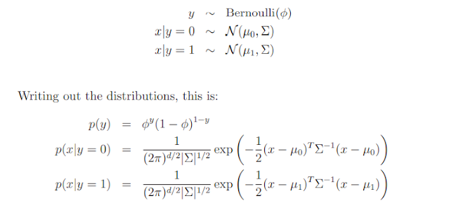Here, the parameters of our model are $φ, Σ, µ0$ and $µ1$. (Note that while there’re two different mean vectors $µ0$ and $µ1$, this model is usually applied using only one covariance matrix $Σ$.) The log-likelihood of the data is given by 

By maximizing $ℓ$ with respect to the parameters, we find the maximum likelihood estimate of the parameters  to be:

Pictorially, what the algorithm is doing can be seen in as follows:

Shown in the figure are the training set, as well as the contours of the two Gaussian distributions that have been fit to the data in each of the two classes. Note that the two Gaussians have contours that are the same shape and orientation, since they share a covariance matrix $Σ$, but they have different means $µ0$ and $µ1$. Also shown in the figure is the straight line giving the decision boundary at which $p(y = 1|x) = 0.5$. On one side of the boundary, we’ll predict y = 1 to be the most likely outcome, and on the other side, we’ll predict $y = 0$.

 GDA and logistic regression

The GDA model has an interesting relationship to logistic regression. If we view the quantity $p(y = 1|x; φ, µ0, µ1, Σ) $ as a function of $x$, we’ll find that it can be expressed in the form 

where $θ$ is some appropriate function of $φ, Σ, µ0, µ1$. This is exactly the form that logistic regression—a discriminative algorithm—used to model $p(y = 1|x)$. When would we prefer one model over another? GDA and logistic regression will, in general, give different decision boundaries when trained on the same dataset. Which is better?

We just argued that if $p(x|y)$ is multivariate gaussian (with shared $Σ$), then $p(y|x)$ necessarily follows a logistic function. The converse, however, is not true; i.e., $p(y|x)$ being a logistic function does not imply $p(x|y)$ is multivariate gaussian. This shows that GDA makes stronger modeling assumptions about the data than does logistic regression. It turns out that when these modeling assumptions are correct, then GDA will find better fits to the data, and is a better model. Specifically, when $p(x|y)$ is indeed gaussian (with shared $Σ$), then GDA is asymptotically efficient. Informally, this means that in the limit of very large training sets (large $n$), there is no algorithm that is strictly better than GDA (in terms of, say, how accurately they estimate $p(y|x)$). In particular, it can be shown that in this setting, GDA will be a better algorithm than logistic regression; and more generally, even for small training set sizes, we would generally expect GDA to better.

In contrast, by making significantly weaker assumptions, logistic regression is also more robust and less sensitive to incorrect modeling assumptions. There are many different sets of assumptions that would lead to $p(y|x)$ taking the form of a logistic function. For example, if $x|y = 0 ∼ Poisson(λ_0)$, and $x|y = 1 ∼ Poisson(λ_1)$, then $p(y|x)$ will be logistic. Logistic regression will also work well on Poisson data like this. But if we were to use GDA on such data—and fit Gaussian distributions to such non-Gaussian data—then the results will be less predictable, and GDA may (or may not) do well.

To summarize: GDA makes stronger modeling assumptions, and is more data efficient (i.e., requires less training data to learn “well”) when the modeling assumptions are correct or at least approximately correct. Logistic regression makes weaker assumptions, and is significantly more robust to deviations from modeling assumptions. Specifically, when the data is indeed non-Gaussian, then in the limit of large datasets, logistic regression will almost always do better than GDA. For this reason, in practice logistic regression is used more often than GDA